Step 3. Selection

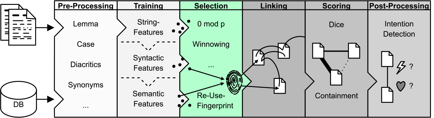
There are roughly sixty different selection strategies in TRACER, which can also be combined. Through Selection we look at the idiosyncrasies or minutiae of the features we’ve computed, thus focusing on fewer features while being faster and more precise. This is the point where we create our ‘fingerprint’ with the core reuse elements we’re interested in. Algorithmically-speaking, through Selection some entries in the KJV.train file will be kicked out. With Selection we’re narrowing down the search by filtering out all irrelevant results. The challenge in this step is to find out what our core elements or minutiae are.

Selection strategies

There are many different selection strategies, including:

• Pruning: maximum or minimum.
  • Maximum pruning cuts out high frequency words (e.g. function words); removing high frequency words reduces computational complexity. For example, if you’re looking at a feature that occurs only 10 times you are comparing one feature with 9 others - this means that you are making 90 comparisons. This is reasonably fast. If you, however, do not prune and have a frequency of 100, you would have to make 900 comparisons. That’s slow.
  • Minimum pruning removes low frequency words (e.g. words with a frequency of 1). Min pruning is used to clear up more space on the desk by reducing the size of the index.
• Term weighting: we give features a weight. Rarer words have a higher weight.
• Frequency classes: you can take the frequency of the most frequent word and divided it by the frequency of the word you want to compare it to.
• Feature dependencies: it makes a comparison between paired features and sees if there are features that tend to co-occur.
• Random selection: random selection of features. Very good if you don’t have a clue about what to expect from your data.

[warning] To update

Winnowing: The selection is made based on the rarest parts of the winnowing window - i.e. the most infrequent features. But in this way function words are not entirely removed, since sometimes they can still be useful. With the winnowing algorithm it’s possible to select features all over the reuse unit and avoid clusters. For example, “To be or not to be that is the question". It would appear that the only interesting word here is ‘question’ but we don’t want to be eliminating all of the rest. Winnowing, with its windows, allows us to pick the lowest ranked feature (in frequency) for every window - so there is a selected feature for every window and features are distributed evenly.

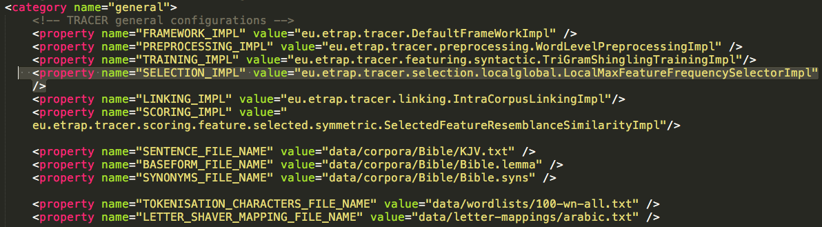
To change the selection strategy in TRACER, locate the Selection strategy in the tracer_config.xml file, as shown in the Figure below.

Different selection strategies require different parameters, and it’s often difficult to compare and decide which strategy works best for a given case. For this reason, we use the Feature Density or, in other words, the comparison between the overall number of features and the number of features selected. The Feature density parameter accepts value ranges between 0 and 1; for, for example, if it is set to 0.8, TRACER will keep 80% of the features and ignore the remaining 20%. Here’s how TRACER computes feature density:

[warning] To update

The feature density F is the quotient of the sum of features in the signature matrix s (with dimensions n, m) and the sum of features in the feature matrix f (with dimensions n, m). The signature matrix s stores 1 to represent the appearance of a given feature in a given reuse unit, but drops features if they appear in only one reuse unit (or a defined threshold). In contrast, the feature matrix f stores 1 to represent the appearance of a given feature in a given reuse unit, but does not drop any feature.

Simply put:

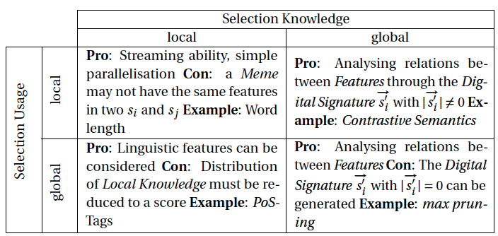
• Global knowledge: Information derived fromthe entire corpus; global knowledge is, for example, the computed feature frequency in a corpus.
• Local knowledge: Information derived from the reuse unit (e.g. a sentence); local knowledge is the context of the reuse unit or, for instance, the length of its words.
• Global usage: Selection is applied to, for example, the entire text or corpus.
• Local usage: Selection is applied to the reuse unit.

These can be combined in the tracer_config.xml file in the following ways:

• localglobal: Local knowledge in a global context. This is the default setting of TRACER and the most used.
• globallocal: Global knowledge in local context.
• globalglobal: Global knowledge in a global context. TRACER treats every reuse unit in the same way but it can easily create empty reuse units.
• locallocal: Local knowledge in a local context. For example, given a certain word-length, TRACER removes from the reuse unit all words that are shorter than the specified length.